
Predictive Maintenance: Vibration Trend, Corrosion Monitor
Predictive maintenance guide to vibration trending and corrosion monitoring methods that reveal equipment degradation weeks before failure.
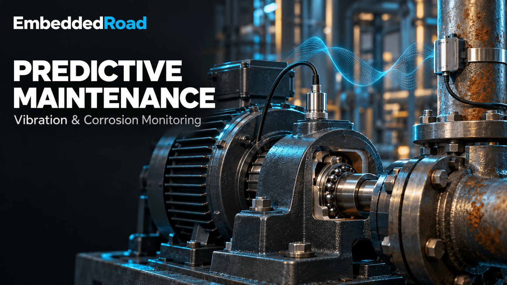
Contents & prerequisites
Prerequisites
Why Predictive Maintenance Matters in Industrial Settings
Unplanned downtime on rotating equipment or pressure-retaining assets costs far more than the repair itself — lost production, secondary damage, and expedited parts shipping routinely multiply the direct cost by 5-10x. Predictive maintenance (PdM) addresses this by watching how a measurement changes over time rather than treating each reading as a pass/fail check.
Reactive vs. Preventive vs. Predictive Strategies
Reactive maintenance repairs equipment after it fails — cheapest in instrumentation cost, most expensive in downtime. Preventive maintenance replaces parts on a fixed schedule regardless of actual condition, which wastes good components and still misses failures that occur early. Predictive maintenance instead uses condition data — vibration spectra, wall thickness, corrosion rate — to estimate remaining useful life and schedule intervention only when degradation trends indicate it's needed.
Cost Reduction Through Early Fault Detection
A bearing with a developing spall typically gives 2-8 weeks of warning in the vibration envelope spectrum before it generates audible noise or heat. Catching it at that stage means a planned bearing swap during a scheduled outage instead of a cascading gearbox failure. The same logic applies to corrosion: a wall-loss trend crossing a retirement-thickness threshold six months out allows a scheduled pipe spool replacement instead of an unplanned shutdown or, worse, a leak.
Equipment Availability and Production Uptime
PdM programs are judged on mean time between failures (MTBF) and overall equipment effectiveness (OEE), not on sensor count. A plant with good trending infrastructure can push scheduled maintenance intervals outward on healthy assets while pulling them in on degrading ones — net availability gain comes from both directions.
Vibration Monitoring: Principles and Trending
Accelerometer Selection and Mounting Techniques
Piezoelectric IEPE (Integrated Electronics Piezo-Electric) accelerometers dominate industrial vibration monitoring due to their wide frequency range (typically 0.5 Hz to 10 kHz for general-purpose units) and low-noise two-wire constant-current interface. Mounting method matters as much as sensor spec: stud-mounting gives the flattest frequency response and highest usable bandwidth, adhesive mounting is acceptable to a few kHz, and magnetic mounts — common for route-based data collection — roll off well below the stud-mounted figure and can introduce mounting resonances. For bearing defect frequencies in the 1-20 kHz envelope band, magnetic mounts are often inadequate; check the datasheet's mounted frequency response curve before committing to a mounting method for a permanent installation.
Frequency Domain Analysis: Bearing Defects and Misalignment Signatures
Time-domain waveforms rarely distinguish fault types; the FFT does. Shaft misalignment (angular or parallel) produces strong energy at 1x and especially 2x running speed, often with high axial vibration relative to radial — a signature distinct from unbalance, which concentrates almost purely at 1x radial. Bearing defects instead generate non-synchronous frequencies tied to bearing geometry: ball pass frequency outer race (BPFO), ball pass frequency inner race (BPFI), ball spin frequency (BSF), and fundamental train frequency (FTF). These are calculated from the bearing's geometry (ball diameter, pitch diameter, contact angle) — look up the formulas and your bearing's specific dimensions in the manufacturer's bearing data sheet rather than relying on generic ratios. Early-stage bearing defects appear as low-amplitude sidebands around these frequencies; by the time they dominate the raw spectrum, the bearing is often near end-of-life.
Envelope Analysis and Demodulation for Early Fault Detection
Raw FFT often buries early bearing fault energy under gear mesh or structural resonance content. Envelope analysis (also called demodulation or high-frequency enveloping) band-pass filters the signal around a structural resonance excited by impacting, then demodulates the envelope and runs a second FFT. This reveals BPFO/BPFI harmonics weeks before they're visible in the raw spectrum, because it isolates the repetitive impact signature from broadband noise.
Establishing Baseline and Alarm Thresholds
A reliable baseline requires 3-5 measurements taken under consistent operating conditions (load, speed, temperature) after commissioning or after any maintenance event that resets wear. Overall vibration severity thresholds from ISO 10816 / ISO 20816 provide a starting point by machine class and mounting type, but they're generic; the more valuable alarms are statistical — typically alert at baseline + 2 standard deviations and alarm at baseline + 4-6x, or at a fixed percentage increase (e.g., 25% over rolling 90-day average) in specific fault-frequency bands. Document the baseline conditions alongside the numbers; a threshold taken at 60% load is not valid at 100% load.
Trend Data Collection and Historical Comparison
Store not just overall RMS but band-limited energy in the specific fault frequencies identified above, sampled at a consistent interval (daily for route-based collection, continuous for online systems). A simple trend table for a pump bearing might look like:
Date        1x_mm/s  2x_mm/s  BPFO_env_gE  Overall_mm/s
2024-01-05  0.8      0.3      0.05         1.4
2024-02-05  0.8      0.3      0.06         1.4
2024-03-05  0.9      0.3      0.11         1.6
2024-04-05  0.9      0.4      0.28         2.1   <- alert
2024-05-05  1.0      0.4      0.61         3.0   <- alarm, schedule replacement
The overall RMS barely moves until April, but the envelope energy at BPFO has already grown 5x by March — this is the early-warning advantage of frequency-specific trending over single-number monitoring.
Corrosion Monitoring Technologies
Electrochemical Probe Methods: Polarization Resistance and LPR
Linear Polarization Resistance (LPR) probes apply a small potential perturbation (typically ±10-20 mV) around the corrosion potential and measure the resulting current to compute polarization resistance, which is inversely proportional to instantaneous corrosion rate via the Stern-Geary equation. LPR gives a real-time rate reading (often updated every few minutes) rather than a cumulative loss figure, making it well suited to catching rate excursions caused by process upsets — a chemical injection failure or a pH swing shows up within the hour, not the next inspection cycle.
Ultrasonic Thickness Measurement for Wall Loss Detection
Ultrasonic thickness (UT) gauging measures remaining wall thickness directly by timing the echo of a sound pulse through the material. Permanently installed UT sensors enable automated wall-loss trending at fixed points, which is more representative of actual pipe condition than electrochemical proxies but updates much more slowly (loss rates are often fractions of a mm/year) and only reports a trailing indicator — by the time thinning is measurable, the metal loss has already occurred.
Coupon-Based and In-Situ Monitoring Approaches
Weight-loss coupons remain the baseline reference method: a metal specimen of known composition and mass is exposed to the process stream for a fixed interval, then removed and weighed to compute an average corrosion rate over that period. Coupons are inexpensive and material-specific but give only a retrospective average — they can't catch a short-duration upset that occurred mid-interval. In-situ electrochemical and UT methods complement coupons by filling in the time resolution coupons can't provide; many plants run both, using coupons for calibration/validation of the continuous methods.
Environmental Factors and Corrosion Rate Prediction
Corrosion rate is highly sensitive to temperature, flow velocity, dissolved oxygen, and pH — a 10°C increase can roughly double rate for many aqueous mechanisms. Any trending model needs process condition tags alongside the corrosion measurement, or an unrelated process upset will look like an electrode fault.
Sensor Integration and Data Acquisition
Accelerometer Output Signal Conditioning
IEPE accelerometers need constant-current excitation (commonly 2-20 mA, check sensor datasheet) and AC-coupling to strip the DC bias before digitization. Signal conditioning modules also provide anti-alias filtering — essential since FFT analysis up to the bearing fault frequencies demands a sample rate at least 2.56x the highest frequency of interest to avoid spectral aliasing corrupting the diagnosis.
Analog and Digital Signal Processing for Trending
Raw waveform capture at the sensor is usually impractical to store continuously; typical architectures compute FFT or envelope spectra on-device or at a gateway and transmit summary bands plus periodic full-spectrum snapshots for diagnostic review.
Real-Time vs. Interval-Based Sampling Strategies
Continuous online monitoring suits critical, expensive machinery (large compressors, turbines) where failure consequence justifies the hardware cost. Route-based interval collection (weekly/monthly handheld data collection) suffices for balance-of-plant pumps and fans where slower fault progression and lower criticality make the labor cost acceptable.
Wireless Transmission and Edge Computing Considerations
Battery-powered wireless vibration nodes trade continuous sampling for power budget — many report band-limited summary values every 15-60 minutes instead of streaming raw waveforms. Edge computation of FFT/envelope features locally reduces radio airtime and battery drain substantially compared to transmitting raw time waveforms. The constraints here overlap heavily with general industrial sensor networking; see the discussion of Industrial IoT (IIoT) vs. Consumer IoT Differences for why industrial deployments favor deterministic, low-duty-cycle protocols over consumer-grade Wi-Fi/BLE patterns.
Building a Predictive Maintenance System
Sensor Placement Strategy Across Equipment Fleet
Place accelerometers at each bearing housing, in both radial (horizontal and vertical) and axial orientations where misalignment or thrust-related faults are a risk. Avoid single-point monitoring on multi-bearing machine trains — a fault on a far bearing can be structurally attenuated before reaching a sensor on the near bearing, producing false negatives. For corrosion, place probes/UT points at known high-risk locations: elbows, dead legs, and flow-regime transitions, not just arbitrary straight-run points.
Data Logging and Trend Storage Requirements
Store time-stamped feature vectors (band energies, overall levels, corrosion rates) indefinitely at a resolution fine enough to compute rate-of-change, with raw spectra retained at reduced frequency (e.g., weekly) for retrospective diagnosis. Tie each record to operating context — load, speed, process temperature — since threshold validity depends on it.
Alert Generation Logic and Notification Workflows
Use layered thresholds: an "alert" state flags the record for review without paging anyone, and an "alarm" state (sustained over N consecutive readings, not a single transient) triggers a maintenance work order. Requiring persistence across multiple readings before alarming is the single most effective way to suppress false positives from transient process conditions.
Integration with Asset Management Platforms
PdM data is only actionable if it reaches a CMMS/EAM as a work order rather than sitting in a historian. Standardized messaging models such as those described in ETSI SmartM2M: oneM2M Architecture and API help normalize how heterogeneous sensor types (vibration, corrosion, temperature) publish into a common resource model that downstream asset systems can subscribe to, rather than building point-to-point integrations per sensor vendor.
Measurement Uncertainty and Calibration in Predictive Systems
Transducer Calibration and Traceability for Trending Reliability
Accelerometer sensitivity drift of even a few percent can masquerade as a real trend if uncorrected. Maintain calibration traceable to a national standard (per ISO 17025 lab practice) on a schedule set by sensor type and criticality, and record calibration date/sensitivity alongside historical data so retroactive correction is possible if drift is discovered.
Environmental Drift and Temperature Compensation
Piezoelectric sensitivity and electrochemical probe response both vary with temperature. Where ambient temperature swings are significant, either apply a compensation curve from the sensor datasheet or normalize trend comparisons to readings taken within a consistent temperature band.
Validation of Trend Algorithms Against Known Failure Modes
Before trusting an alarm threshold in production, validate it against at least one documented failure history — bearing teardown records correlated against the envelope trend, or UT thickness logs correlated against an actual leak event — to confirm the algorithm would have given adequate lead time.
Implementation Case Studies and Best Practices
Rotating Equipment Monitoring in Process Plants
A typical pilot starts with 10-20 critical pumps and compressors fitted with permanently mounted accelerometers, feeding envelope and band-energy trends into a historian with layered alarms. Success is measured by comparing detected lead time against historical failure records for the same asset class.
Pipeline and Pressure Vessel Corrosion Surveillance
Combining LPR probes for rate response with periodic UT surveys for absolute thickness confirmation gives both the fast feedback and the ground-truth check needed to trust automated corrosion alarms over a multi-year asset life.
Scaling from Pilot Programs to Facility-Wide Deployment
Moving from a pilot to fleet-wide coverage raises data volume and network design concerns that resemble broader facility instrumentation problems — the sub-metering and integration patterns discussed in Energy Management IoT: Sub-Metering, BEMS Integration are a useful reference for scaling data aggregation, since both domains face the same challenge of consolidating many distributed low-bandwidth sensor feeds into a single trending and alarming backbone without overwhelming the historian or the maintenance team with alerts.
Learning
Sign in to track your progress.
Evidence
Public projects engineers linked to Predictive Maintenance: Vibration Trend, Corrosion Monitor.
No engineer has linked a project to this topic yet. Built something that proves it? Add the project and tag it with instrumentation-measurement-predictive-maintenance-vibration-trend-corrosion-m — it then shows here and on your public profile.