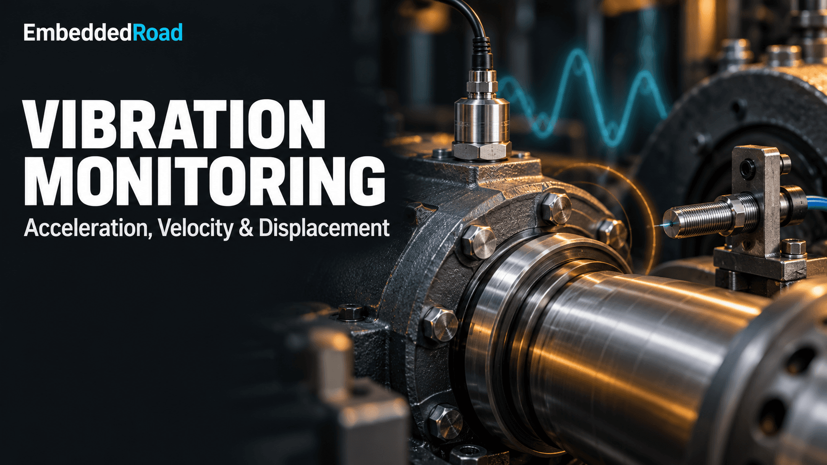
Vibration Monitoring: Velocity, Acceleration, Proximity Probe

Why Vibration Monitoring Matters in Predictive Maintenance

Unplanned downtime on rotating equipment costs far more than the repair itself — lost production, secondary damage, and expedited parts shipping routinely multiply the direct cost by 5-10x. Vibration monitoring is the primary sensing modality for catching mechanical degradation before it becomes a failure event, because almost every mechanical fault — imbalance, misalignment, bearing wear, gear mesh defects, rotor rubs — injects energy into the structure at characteristic frequencies long before it produces audible noise or measurable performance loss.

Early fault detection in rotating machinery

A bearing spall, a bent shaft, or a loose foundation bolt each modulates the vibration signature in a distinct way. Imbalance shows up as a strong 1x running-speed component. Misalignment adds 2x and sometimes axial components. Bearing defects generate repeatable impact frequencies tied to raceway and rolling-element geometry, often at several kHz, well above running speed. The fault's signature frequency band dictates which transducer can actually see it — this is the central engineering decision this article addresses.

Condition-based maintenance vs. fixed intervals

Fixed-interval maintenance replaces or services a component on a calendar or runtime schedule regardless of actual condition, which either wastes good remaining life or misses degradation that develops faster than expected. Condition-based maintenance (CBM) instead trends a measurement — RMS velocity, peak acceleration, shaft displacement — against a baseline and intervenes when the trend crosses a threshold. CBM requires sensors stable enough that a trend change means the machine changed, not that the sensor drifted.

Cost-benefit analysis of vibration diagnostics

A single accelerometer and signal-conditioning channel costs a small fraction of one unplanned outage on a critical asset. The harder cost question is instrumentation density: permanently wired proximity probes on every bearing of a multi-million-dollar turbine are justified; the same approach on a balance-of-plant pump is not, where a route-based handheld accelerometer survey is more economical.

Acceleration-Based Vibration Measurement

Piezoelectric accelerometer principles and frequency response

A piezoelectric accelerometer uses a seismic mass preloaded against a piezoelectric crystal (quartz or ceramic). Inertial force from the mass under acceleration stresses the crystal, which generates a charge proportional to force, and therefore proportional to acceleration (F = ma). The sensor has a usable flat region bounded below by its low-frequency rolloff (set by the charge amplifier's input time constant, typically a few Hz to tens of Hz) and above by the mechanical resonance of the mass-spring system, often in the 20-30 kHz range for general-purpose industrial units. Manufacturers typically specify the usable range as roughly one-third to one-fifth of the mounted resonant frequency — confirm the exact figure against the specific sensor's datasheet rather than assuming a number.

High-frequency transient capture for bearing defects

Bearing defect frequencies and gear mesh harmonics live in the kHz range, and the impulsive nature of a spall strike produces a short, high-amplitude transient that a velocity or displacement sensor's lower bandwidth simply cannot resolve. Acceleration is the only one of the three quantities with enough high-frequency response to catch these events early, which is why envelope demodulation (bandpass filter the raw acceleration, rectify, then FFT the envelope) is a standard bearing-diagnostic technique built on accelerometer data.

Units, mounting considerations, and signal conditioning

Acceleration is reported in g (9.81 m/s²) or m/s². Mounting method directly trades off against usable frequency range: a stud-mounted sensor on a flat machined pad preserves resonance up into the tens of kHz; a magnetic mount drops usable bandwidth to a few kHz; a hand-held probe is suitable only for low-frequency trending below roughly 1 kHz. Piezoelectric sensors require either a charge amplifier or, more commonly in industrial practice, an integrated IEPE (constant-current powered) circuit that converts charge to a low-impedance voltage inside the sensor housing, which tolerates longer cable runs without the signal degradation a raw charge output would suffer.

When to choose acceleration monitoring

Choose acceleration when the fault of interest is high-frequency: rolling-element bearings, gear mesh, blade-pass, or any impact-type defect. It's the default choice for pumps, fans, motors, and gearboxes with rolling-element bearings.

Velocity-Based Vibration Measurement

Geophone and electromagnetic velocity transducers

A classic velocity transducer (geophone-style) suspends a coil in a magnetic field; relative motion between coil and magnet induces a voltage directly proportional to velocity. These are self-generating (no external power) but mechanically limited to roughly 10 Hz to 1-2 kHz and are heavier and more fragile than accelerometers, so most modern installations instead derive velocity electronically.

Integration from acceleration and differentiation relationships

Velocity is the time integral of acceleration; displacement is the time integral of velocity. In practice, nearly all "velocity" sensors sold today are IEPE accelerometers with an analog or digital integrator built into the signal path. Integration in the frequency domain divides amplitude by angular frequency (ω = 2πf), which suppresses high-frequency content and amplifies low-frequency noise and DC drift — so integrated-velocity signal chains need a high-pass filter to keep the integrator from railing. This relationship is also why velocity is naturally less sensitive to the high-kHz bearing defect energy that dominates raw acceleration: the integration step itself acts as a low-pass filter on the physical quantity of interest.

Worked relationship for a pure sinusoidal vibration at frequency f:

a(t) = A·sin(2πft)
v(t) = -(A / (2πf))·cos(2πft)     → v_peak = a_peak / (2πf)
d(t) = -(A / (2πf)^2)·sin(2πft)   → d_peak = a_peak / (2πf)^2

Example: a machine vibrating at 1 g peak (9.81 m/s²) at 50 Hz has a peak velocity of 9.81 / (2π·50) ≈ 31.2 mm/s, and a peak displacement of 31.2 / (2π·50) ≈ 0.099 mm. Note how the same acceleration amplitude translates to a much larger velocity number at low frequency than at high frequency — this is precisely why velocity is the preferred broadband severity metric for mid-speed machinery and displacement is preferred for very low frequency shaft motion.

ISO 20816 velocity thresholds for machine health zones

ISO 20816 (successor to ISO 10816) defines RMS velocity zones (A/B/C/D, good through unacceptable) as a function of machine class — small machines, medium machines on rigid vs. flexible foundations, large turbomachinery, etc. The exact mm/s boundaries differ by machine class and mounting, so pull the specific table for the asset class from the current ISO 20816 part rather than relying on a remembered number; using the wrong class's thresholds is a common and avoidable field error.

Broadband energy analysis and trend monitoring

Overall RMS velocity in the 10 Hz-1 kHz band correlates well with mechanical "roughness" across imbalance, misalignment, and looseness faults, which is why it's the default single-number trend metric in route-based CBM programs — simple to compute, standardized, and directly comparable against ISO zone boundaries machine to machine.

Proximity Probe (Eddy-Current) Displacement Measurement

Non-contact capacitive/inductive sensing principles

An eddy-current proximity probe drives a coil with a high-frequency RF signal; a conductive target (the shaft) in the resulting field develops eddy currents that load the coil, changing its impedance in proportion to the gap distance. The driver electronics demodulate this into a DC voltage proportional to gap — typically on the order of a few hundred mV/mil or several V/mm, calibrated per target material.

Radial and axial shaft displacement monitoring

Two radial probes mounted 90° apart at a bearing reveal orbit shape (shaft centerline motion), while an axial probe against a thrust collar tracks axial position for thrust-bearing wear monitoring. Unlike accelerometers and velocity sensors, which measure casing motion, proximity probes measure the shaft directly relative to the bearing housing — the quantity that actually matters for rotor-to-stator clearance.

Turbomachinery applications and rotor dynamics

On fluid-film (journal) bearing machines — large turbines, compressors, high-speed pumps — the bearing housing itself may barely vibrate even while the shaft orbits wildly inside its clearance, because the oil film decouples casing motion from shaft motion. Casing-mounted accelerometers and velocity sensors are effectively blind to this; only a shaft-relative proximity probe sees it. This is the central answer to why proximity probes outperform contact-based transducers on high-speed turbomachinery: they measure the right reference frame, not just a different frequency band.

Probe calibration, gap distance, and material effects

Eddy-current probes must be calibrated against the specific target material (steel alloys shift calibration slope versus the factory reference, usually 4140 steel) and operated within a linear gap range, commonly a few tens of mils, bounded below by contact risk and above by sensitivity rolloff. Shaft surface finish, plating, and even residual magnetism can introduce glitch (non-vibration electrical noise riding on the signal), so gap calibration and runout checks on a lathe or V-block fixture before installation are standard practice, not optional.

Comparative Analysis: Acceleration vs. Velocity vs. Displacement

Frequency domain sensitivity and machine type suitability

High frequency (kHz, bearing/gear defects): acceleration. Mid frequency (10 Hz-1 kHz, imbalance/misalignment, rolling-element bearing machines): velocity. Low frequency (sub-10 Hz, shaft orbit, fluid-film bearings): displacement via proximity probe. The physics of integration (dividing by ω) and the physical reference frame (casing vs. shaft) together determine which sensor sees a given fault.

Overlapping use cases and hybrid monitoring strategies

Large turbomachinery trains commonly carry all three: proximity probes for shaft radial/axial position (API 670 compliant installations), casing accelerometers for high-frequency bearing and gear diagnostics, and derived velocity for overall severity trending against ISO 20816. No single sensor type is redundant; each covers a distinct failure mode.

Signal processing trade-offs and noise immunity

Accelerometer signals need careful high-frequency anti-alias filtering ahead of digitization; integrated velocity needs high-pass filtering to prevent drift; proximity probes need shielded cabling and gap-voltage checks because the raw signal is DC-coupled and any cable damage shows up as a gap offset rather than an obvious fault.

Selection matrix for industrial equipment classes

Rolling-element bearing pumps/fans/motors: accelerometer primary, velocity for trending. Fluid-film bearing turbines/compressors: proximity probes primary (per API 670 for critical machinery), accelerometers supplementary on the casing. Reciprocating compressors: a mix, often with additional crank-angle-referenced measurements beyond the scope of these three sensor types alone.

Signal Conditioning and Data Acquisition

Amplification, filtering, and ADC requirements

IEPE accelerometers need a constant-current power source (typically 2-20 mA) and a coupling capacitor to strip the DC bias before amplification. Anti-alias low-pass filtering ahead of the ADC must be set below half the sample rate per Nyquist, and because bearing diagnostics push into the kHz range, sample rates of 20-50 kHz per channel are common on dedicated vibration DAQ, well above what a general-purpose process historian channel provides. The gain-and-filter stage is conceptually the same amplifier and divider-network design problem covered in voltage divider and current divider rules, and the frequency-dependent loading effects a long sensor cable introduces are usefully analyzed with two-port network parameters when characterizing cable and conditioning-amplifier interaction.

Real-time vs. batch trending and FFT analysis

Protection systems (trip on overall vibration for a turbine) need real-time, low-latency RMS computation in hardware or firmware. Diagnostic systems can batch-capture time waveforms periodically and compute FFTs offline or on an edge device, trading latency for deeper spectral resolution.

Integration with industrial IoT platforms for remote monitoring

Route-based or continuously wired vibration data increasingly feeds industrial IoT gateways that forward FFT summaries or alarm flags to a cloud historian rather than raw high-rate waveforms, to conserve bandwidth. The constraints here — determinism, security posture, and data volume — differ substantially from consumer sensor networks, a distinction covered in Industrial IoT vs. Consumer IoT differences. Where vibration data is combined with power consumption trending for overall asset efficiency, it often shares infrastructure with systems built for energy management IoT sub-metering and BEMS integration.

Alarm thresholds and fault classification

Alarm setpoints should be derived from the applicable ISO 20816 zone boundary for the machine class plus a baseline-relative alert (commonly 2-3x the machine's own established baseline RMS) rather than a single absolute number copied from another asset — two nominally identical pumps on different foundations can have legitimately different baselines.

Installation, Calibration, and Best Practices

Mounting methods and their impact on measurement accuracy

As noted above, stud mounting preserves the highest usable frequency range; adhesive pads and magnets trade bandwidth for installation speed. Always document mounting method alongside the data, since a trend break can result from a mounting change rather than a machine fault.

Baseline establishment and measurement uncertainty

A baseline should be collected over multiple runs across normal operating conditions (load, speed, temperature) to capture natural variance before any alarm threshold is set; a single reading mistaken for "normal" can hide an already-developing fault.

Periodic verification and traceability requirements

Accelerometers and proximity probe systems should be periodically checked against a traceable shaker or calibrated reference per the manufacturer's recommended interval, with calibration certificates retained for audit in regulated industries (API 670 environments in particular expect documented traceability).

Documentation and asset management integration

Sensor serial numbers, mounting location, orientation, and calibration dates belong in the CMMS/asset record tied to each measurement point, so a future trend anomaly can be checked against hardware history before being escalated as a mechanical fault.