
Gain-Bandwidth Product (GBW): 1 MHz, 10 MHz Devices
Learn how gain-bandwidth product sets op-amp speed limits, calculate closed-loop bandwidth, and choose between 1 MHz and 10 MHz devices.
Contents & prerequisites
What is Gain-Bandwidth Product?
Definition and fundamental relationship
Gain-bandwidth product (GBW) is the single number that tells you how an op-amp trades gain for speed. For a voltage-feedback op-amp with a dominant single-pole open-loop response, the product of closed-loop gain and closed-loop bandwidth is approximately constant:
GBW ≈ A_CL × f_CL
If you know the GBW and the gain you need, you can solve directly for the bandwidth you'll get. That's the whole point of the spec: it lets you predict performance in a configuration the datasheet never explicitly characterizes, as long as you stay in the region where the single-pole approximation holds (typically from the dominant pole frequency up to where second-order effects — slew rate, parasitic poles — start to dominate).
Why GBW is a fixed characteristic of op-amps
GBW is set by the internal compensation of the amplifier, not by how you wire the feedback network. A typical op-amp — see the general topology discussed in Two-Stage Op-Amp: Differential Input + Common-Source Output — has a high-gain first stage followed by a second gain/output stage, with a compensation capacitor deliberately placed to create one dominant low-frequency pole. That capacitor, combined with the output resistance of the stage driving it and the transconductance of the input pair, fixes the location of the dominant pole and the open-loop unity-gain crossover frequency. The product of open-loop DC gain and the dominant pole frequency equals the unity-gain frequency — and that unity-gain frequency is what's commonly marketed as "GBW." It's baked into the silicon: changing it requires changing the compensation capacitor or the transconductance, which the manufacturer fixes at fabrication (or, in rare adjustable-compensation parts, with an external pin). You cannot get more GBW out of a 1 MHz part by changing your feedback resistors — you only move where on that fixed open-loop curve your closed-loop pole lands.
Closed-loop bandwidth vs open-loop bandwidth
Open-loop bandwidth is the frequency at which the op-amp's raw, no-feedback gain has rolled off by 3 dB from DC — often just a few hertz to a few tens of hertz for a general-purpose part, because open-loop DC gain is enormous (80–120 dB). Closed-loop bandwidth is what you actually get once you wrap feedback around the amplifier to set a defined gain; it's dramatically higher than the open-loop corner because feedback trades away gain for bandwidth along that constant-GBW line. The whole discipline of op-amp speed selection is about deciding where on that trade-off curve your application needs to sit.
1 MHz GBW Devices: Characteristics and Trade-Offs
Typical applications and use cases
Devices with 1 MHz GBW are the workhorses of low- to mid-frequency signal conditioning: sensor buffering, DC and low-frequency instrumentation front ends, audio-band filtering (below roughly 20 kHz), precision DC gain stages, and general-purpose op-amp duties in mixed-signal boards where the signal of interest never approaches the hundreds-of-kHz range.
Advantages: power consumption and noise performance
Lower GBW parts are typically biased with lower internal currents, since bandwidth and bias current trade off directly through transconductance. That means lower quiescent supply current, less self-heating, and — importantly — often lower broadband noise, since many noise sources scale with bandwidth: wideband amplifiers integrate more noise power over their larger pass-band, so an unnecessarily fast op-amp can degrade your total output noise even if its noise density per Hz looks equivalent on the datasheet.
Limitations in high-speed signal processing
The ceiling is sharp: once your required signal bandwidth times your required gain approaches 1 MHz, you're out of margin. Phase margin erodes as you approach the GBW limit, slew rate (a related but separate spec) may also become the binding constraint for large-amplitude fast signals, and any attempt to push gain higher at a given bandwidth, or bandwidth higher at a given gain, simply isn't available from the part.
Common device examples and specifications
Classic 1 MHz-class GBW parts include general-purpose single/dual/quad op-amps commonly used for audio and instrumentation — check the specific datasheet for exact GBW, input noise density, and slew rate, since "around 1 MHz" parts vary from roughly 0.5 MHz to 1.5 MHz depending on process and supply voltage.
10 MHz GBW Devices: When You Need More Speed
Audio and instrumentation applications
A 10 MHz device becomes attractive once you need gain and bandwidth simultaneously — a ×20 instrumentation gain stage that must still pass 100 kHz content, or a higher-order active filter where multiple gain stages each eat into the available margin. Audio applications pushing into ultrasonic measurement, high-gain photodiode transimpedance stages, or fast peak detectors are typical candidates.
Wider bandwidth requirements and slew-rate considerations
Choosing by GBW alone is a trap: a 10 MHz part with a mediocre slew rate will still distort large-signal fast edges even though its small-signal bandwidth looks fine. Always check slew rate against your required output swing and frequency: for a sinusoid, the minimum slew rate needed is 2π × f × V_peak. GBW governs small-signal response; slew rate governs large-signal response — you need both specs to clear your requirement.
Power dissipation and thermal concerns
Higher GBW parts draw more quiescent current to achieve the higher transconductance and bandwidth, which raises supply current draw across every channel on the board — significant in battery-powered or high-channel-count designs — and raises die temperature, which can shift offset voltage and bias current drift specs if you're not budgeting thermal margin.
Common device examples and specifications
10 MHz-class GBW parts span general-purpose fast op-amps up to instrumentation-grade fast amplifiers; again, consult the specific datasheet for GBW, slew rate, and input-referred noise, since parts marketed near "10 MHz" range from about 8 MHz to 20 MHz GBW across different process nodes and supply conditions.
GBW Trade-Off: Gain vs Bandwidth
Calculating maximum closed-loop bandwidth from GBW
For a 1 MHz GBW op-amp configured for closed-loop gain of ×100:
f_CL = GBW / A_CL = 1,000,000 Hz / 100 = 10,000 Hz = 10 kHz
So a ×100 gain stage built from a 1 MHz part gives you only 10 kHz of closed-loop bandwidth — fine for audio, unusable for a 50 kHz instrumentation signal. Swap in a 10 MHz part at the same gain and you get 100 kHz, a 10× margin improvement, at the cost of higher supply current and noise bandwidth.
Inverting and non-inverting configuration impacts
The formula above is exact for a non-inverting stage, where closed-loop gain A_CL = 1 + R_f/R_in and the feedback factor β = 1/A_CL sets the crossover directly. For an inverting stage, the noise gain (not the signal gain) is what determines bandwidth: A_noise = 1 + R_f/R_in, which is larger than the signal gain −R_f/R_in for small R_in. Always compute bandwidth from noise gain, not signal gain, or you'll overestimate your available bandwidth in inverting designs. Picking the actual resistor values for R_f and R_in follows the same series/parallel reasoning covered in Series and Parallel Resistor Combinations.
Stability margins and feedback factor
Phase margin depends on where the closed-loop pole (set by GBW × β) falls relative to any second, parasitic poles in the open-loop response (from input capacitance, feedback network capacitance, or load capacitance). High feedback factor (low gain) pushes the closed-loop crossover higher, closer to those second poles, which erodes phase margin and can cause peaking or ringing even though the DC gain and nominal GBW look adequate on paper.
Design equations for fixed-gain amplifiers
For a target closed-loop bandwidth f_target at gain A, the minimum GBW you need is:
GBW_min = A × f_target × margin_factor
where margin_factor (commonly 2–5×) covers phase margin degradation, process variation on GBW itself, and headroom for parasitic poles — don't design right at the calculated edge.
Practical Design Considerations
Selecting GBW for your application requirements
Start from the signal's highest frequency component and the gain you must apply, compute the raw GBW_min, apply your margin factor, then pick the lowest-GBW part that clears it — over-speccing wastes power and raises noise bandwidth for no benefit.
Frequency response and phase margin
Check the datasheet's phase margin at your actual closed-loop gain, not just the unity-gain stability spec; many op-amps are only unconditionally stable above a minimum gain, and running them at lower gain than specified invites oscillation.
Input impedance and output impedance effects
The feedback network's resistor values interact with the op-amp's input capacitance to form an extra pole — relevant when you model the complete loop as a two-port, as described in Two-Port Network Parameters: Z, Y, H, ABCD — and output impedance rises with frequency as open-loop gain rolls off, interacting with cable or load capacitance to further shift the effective loop response.
Component selection and layout impact
Stray PCB capacitance across feedback resistors, long feedback traces, and unterminated output lines all add parasitic poles that matter far more at 10 MHz GBW than at 1 MHz, simply because the usable signal frequencies are higher and the margin to the next parasitic pole is smaller.
Frequency Response and Stability
Bode plot interpretation for different GBW devices
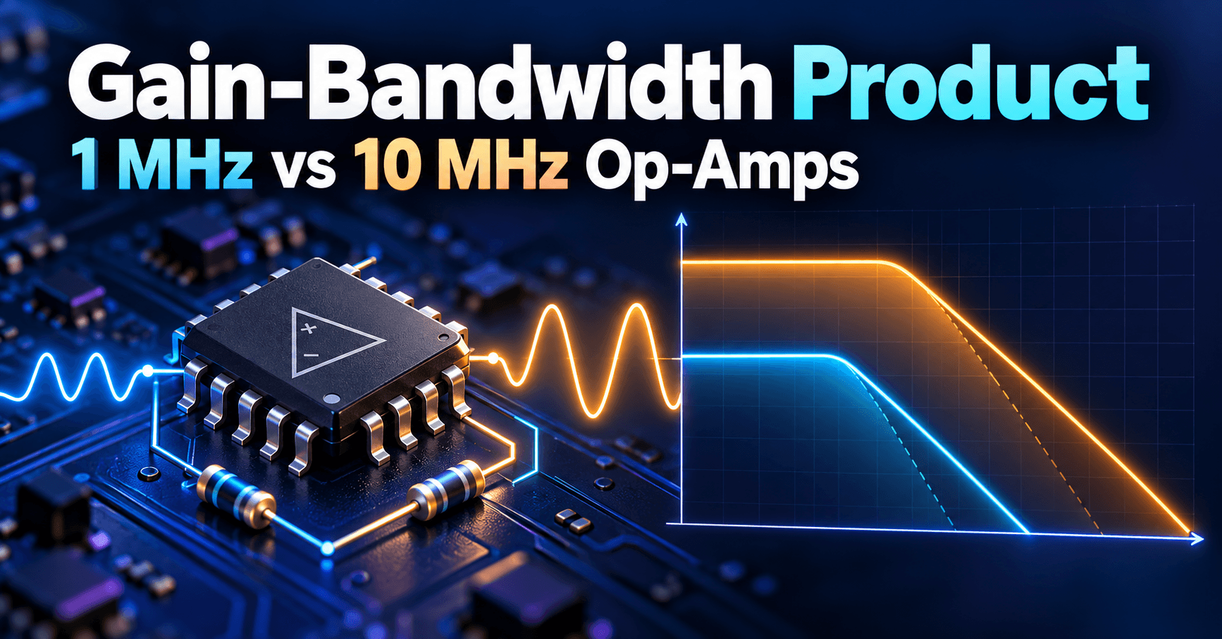
On a Bode plot, GBW sets the single-pole roll-off line at −20 dB/decade from the open-loop DC gain down through unity gain at the GBW frequency; your closed-loop gain line (horizontal, set by feedback) intersects that roll-off at the predicted closed-loop bandwidth — a 10 MHz part's roll-off line sits a decade to the right of a 1 MHz part's, shifting every intersection point correspondingly.
Compensation networks and pole placement
Internal compensation in both device classes places the dominant pole low enough that a single pole dominates up to crossover; external compensation (feedforward caps, snubber networks) can be added by the designer to tame a second pole introduced by capacitive loads, especially on faster parts where that second pole sits closer to the crossover frequency.
Transient response and ringing
A closed-loop pole close to a parasitic second pole shows up in the time domain as overshoot and ringing on a step response, even when the Bode plot phase margin looks marginally acceptable — always verify with a transient simulation or bench step test, not just the frequency-domain margin number.
Overshoot prediction from GBW and feedback
For a well-behaved single-pole-dominant closed loop, percent overshoot correlates with phase margin: roughly 45° phase margin gives noticeable overshoot (~20%), while 60–65° gives a nearly critically damped response with minimal overshoot — use this as a rule of thumb when deciding how much margin_factor headroom to add above the bare GBW_min calculation.
Comparison Table and Selection Guide
1 MHz vs 10 MHz feature summary
| Parameter | 1 MHz class | 10 MHz class |
|---|---|---|
| Typical quiescent current | Lower | Higher |
| Noise bandwidth | Narrower | Wider |
| Max gain at 10 kHz BW | ~100 | ~1000 |
| Max gain at 100 kHz BW | ~10 | ~100 |
| Typical fit | Audio, DC instrumentation | Wideband, high-gain fast stages |
Application matching decision tree
Compute A × f_signal; if it's comfortably under 1 MHz with 2–5× margin, use a 1 MHz part. If it lands between roughly 1 MHz and 10 MHz with margin, move to the 10 MHz class. If it exceeds 10 MHz, you're into a faster device family entirely and need to re-run this same calculation against that part's GBW.
Cost, power, and performance trade-offs
10 MHz parts aren't dramatically more expensive at the component level in most catalogs, but the system-level cost is current draw (more channels, more battery drain, more heat) and noise bandwidth (more integrated output noise unless you add post-filtering) — paying for speed you don't use is a recurring, often invisible design tax.
Migration paths between device classes
Because both classes are typically pin-compatible within a given package family, migrating from a 1 MHz to a 10 MHz part for a bandwidth upgrade is often a drop-in swap — but re-check phase margin and output capacitive load tolerance before committing, since the faster part's reduced margin to parasitic poles can turn a previously stable board into a marginally stable one.
Learning
Sign in to track your progress.
Evidence
Public projects engineers linked to Gain-Bandwidth Product (GBW): 1 MHz, 10 MHz Devices.
No engineer has linked a project to this topic yet. Built something that proves it? Add the project and tag it with analog-electronics-gain-bandwidth-product-gbw-1-mhz-10-mhz-devices — it then shows here and on your public profile.