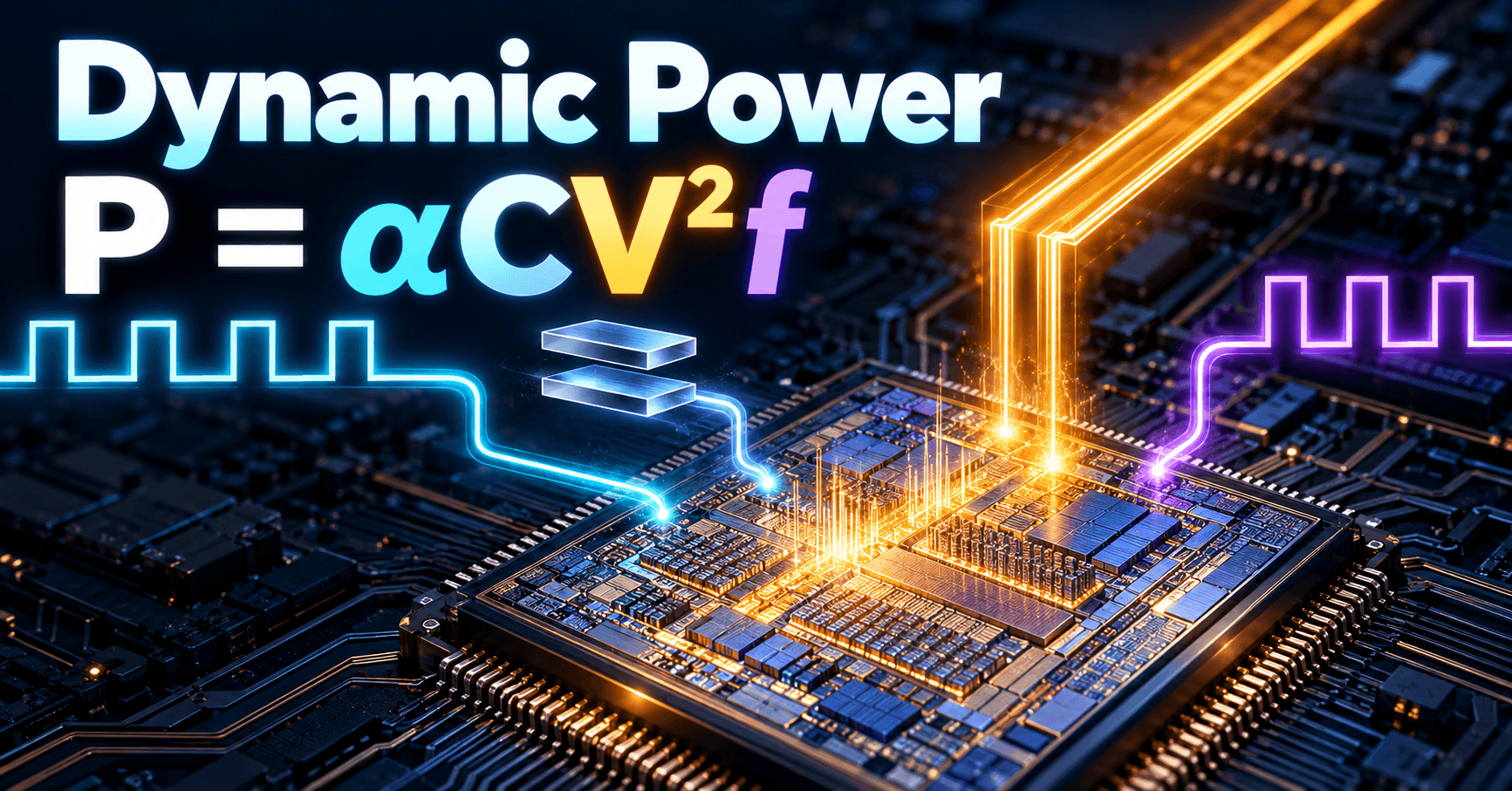
Dynamic Power: P = α C V² f (Activity, Cap, Voltage, Freq)

The Four Levers of Dynamic Power

Why P = αCV²f matters in chip design

Every digital design team that has ever missed a thermal budget has stared at this equation on a whiteboard. P = αCV²f is the single most useful back-of-envelope tool for predicting how much switching power a CMOS block will burn, and it is the reason power architects fight over voltage rails before they fight over clock trees. The formula captures dynamic power only — the energy spent charging and discharging capacitive nodes every time a gate switches. It excludes static leakage, which is a separate mechanism tied to subthreshold conduction and junction effects (see Reverse Bias: Leakage Current, Breakdown Mechanisms for how that term behaves independently of switching activity). In modern sub-10nm processes leakage is no longer a footnote, but dynamic power still dominates during active compute, so this model remains the first filter for any power budget review.

Breaking down each term: activity, capacitance, voltage, frequency

Each symbol is a lever a designer can pull:

• α — the fraction of gates that actually toggle in a given clock cycle, a number between 0 and 1.
• C — the total switched capacitance: gate, junction, and wire load.
• V — the supply voltage swing across the switching node.
• f — the clock frequency driving the switching events.

Power is the product of all four, but they are not equally expensive to change, and they are not independent — lowering V often forces you to lower f too, which is exactly the coupling that makes voltage/frequency scaling (DVFS) a single lever rather than two.

Quadratic voltage dependence and its design implications

The V² term means a 10% voltage cut yields roughly a 19% power cut, while a 10% frequency cut yields only a 10% power cut. This asymmetry is why voltage is the first thing a power architect negotiates and frequency is the second.

Activity Factor (α): The Hidden Multiplier

What activity factor really measures

α is not "percent of transistors," it's the expected number of 0→1 and 1→0 transitions per node per clock cycle, normalized to a 0–1 (sometimes 0–2) scale. A node that toggles every cycle has α ≈ 1. A node that toggles once every 20 cycles has α ≈ 0.05.

How switching statistics affect power consumption

Because power scales linearly with α, a datapath that's busy 100% of the time costs roughly 10x more dynamic power than the same logic running at 10% utilization — the same silicon, radically different power draw depending on the data stream feeding it.

Why not all transistors toggle every cycle

A 64-bit adder processing mostly small numbers won't toggle its upper bits often. A barrel shifter performing a 1-bit rotate activates a different, much smaller subset of its internal mux tree than one performing a 31-bit rotate on a 32-bit word — the switched capacitance for the same block varies by workload, not just by design.

Connection to real workloads vs. worst-case assumptions

Worst-case α = 1 is the number you use for thermal design (peak dynamic power, the figure that determines whether your heatsink and VRM survive a pathological workload). Average α, measured from real traffic traces or RTL simulation with realistic stimulus, is the number you use for battery life and typical-case thermal throttling decisions. Confusing the two is a classic spec-sheet mistake: a chip rated for 5W peak dynamic power might average 1.5W on real code, and designing the power delivery network for the wrong number wastes board area or causes brownouts.

Capacitance (C): Load and Parasitic Effects

Gate oxide and junction capacitance contributions

Every MOSFET gate presents oxide capacitance to whatever drives it, and every diffusion node presents junction capacitance to the substrate. These are fixed by process node and transistor sizing chosen at synthesis/place-and-route time.

Interconnect parasitics and their scaling challenges

As geometries shrink, wire capacitance per unit length doesn't shrink proportionally with gate capacitance — wires get thinner and closer together, so coupling capacitance actually becomes a larger fraction of total C. At advanced nodes, interconnect can account for 30–50% of switched capacitance on long buses; check your foundry's parasitic extraction deck for node-specific numbers rather than assuming a ratio.

Fan-out impact on effective capacitance

A gate driving four downstream inputs presents roughly four times the load capacitance of one driving a single input. High fan-out nets (clock trees, reset trees, shared buses) are prime targets for buffer insertion specifically to manage this term.

Design trade-offs between logic depth and capacitive load

Flattening logic into wider, shallower structures reduces critical path depth but increases fan-out and total capacitance; deep pipelines reduce per-stage C but add flop capacitance and clock load. Neither is strictly cheaper — it's a workload-dependent trade worked out in synthesis constraints.

Voltage (V²): The Dominant Optimization Lever

Why voltage scaling delivers exponential power savings

The squared term means voltage cuts compound: dropping Vdd from 1.0V to 0.8V (a 20% cut) saves roughly 36% of dynamic power, before even touching frequency. No other single parameter in the equation offers that leverage.

Supply voltage vs. threshold voltage constraints

You can't scale Vdd arbitrarily low. As Vdd approaches the transistor's threshold voltage (Vt), switching speed collapses and subthreshold leakage (governed by the same physics discussed in reverse-bias leakage analysis) starts to dominate, flipping the power equation from dynamic-dominant to static-dominant. Process design kits specify a minimum operating voltage (Vmin) below which timing closure and reliability margins are no longer guaranteed — that number lives in your foundry's PDK, not in this article.

Frequency scaling as a side effect of lower voltage

Gate delay is roughly proportional to Vdd/(Vdd−Vt)^α_sat, so lower voltage means slower gates, which means you must lower the achievable clock frequency to keep timing closed. This is why voltage and frequency scale together in real silicon rather than independently.

Trade-offs between voltage reduction and timing slack

If your design has positive timing slack at the target frequency, you can often lower voltage until that slack is consumed, capturing power savings for free. This is the principle behind adaptive voltage scaling (AVS), where on-chip delay monitors find the minimum voltage that still meets timing, cycle by cycle.

Frequency (f): Performance vs. Power Bandwidth

Linear relationship between clock frequency and power

Unlike voltage, frequency scales dynamic power linearly — double the clock, double the switching power, assuming α and C stay constant.

Dynamic frequency scaling (DVFS) strategies

Because voltage and frequency are coupled, real systems implement DVFS: a set of discrete operating points (V, f) pairs, each validated for timing closure, that the OS or power management firmware selects based on workload demand. Mobile SoCs commonly expose a dozen or more such points; the specific table lives in your platform's power management IC datasheet.

Idle state power and always-on overhead

Even at f = 0 for a given block, clock distribution networks and always-on domains (wake-on-event logic, RTC, sensor hubs) keep consuming leakage and sometimes residual switching power — relevant to any system doing fine-grained duty cycling, including the kind of metering logic discussed in Energy Management IoT: Sub-Metering, BEMS Integration.

Task scheduling to minimize frequency demand

Race-to-idle (run fast, finish, then drop to a deep sleep state) often beats running slow-and-steady, because sleep states cut both f and V to near zero, while a moderate frequency reduction only buys linear savings while the task is still active.

Practical Design Strategies for Power Reduction

Comparative effectiveness: voltage vs. frequency vs. activity reduction

Ranked by typical ROI: voltage reduction (quadratic, but constrained by Vmin), activity reduction via clock/power gating (linear, but can approach zero for idle blocks), frequency reduction (linear, constrained by performance requirements). Capacitance reduction is largely a one-time architectural decision locked in at RTL/physical design, not a runtime lever.

Power budgeting and design-phase estimation

Early in the design flow, estimate P = αCV²f per block using RTL activity simulation (toggle counts from testbench traces) and capacitance extracted from a representative standard-cell library, before layout parasitics exist. This gives a budget to allocate across blocks before committing to floorplan.

Power gating and clock gating techniques

Clock gating stops the clock to idle registers, driving effective α toward zero for that domain without touching voltage. Power gating goes further, disconnecting Vdd entirely via header/footer switches, eliminating both dynamic and leakage power for unused blocks — at the cost of wake-up latency that must be budgeted into real-time requirements.

Measurement and validation in silicon

Post-silicon, validate the model by measuring supply current at known (V, f) operating points under controlled workloads, then back-solving for effective α·C. Discrepancies against the pre-silicon estimate usually point to either underestimated interconnect parasitics or activity patterns in real firmware that differ from simulation stimulus.

Real-World Example: Mobile vs. Server Workloads

How activity factor differs across use cases

A phone SoC idling on a home screen might run core logic at α well below 0.1, while a server CPU under sustained load approaches α near 1 across its execution units — the same silicon, radically different power envelopes.

Voltage-frequency operating points in practice

Mobile platforms expose many low-power DVFS points optimized for battery life at modest frequency; server parts often run fewer, higher-voltage points optimized for sustained throughput, accepting a steeper power curve because they're wall-powered.

Power envelope constraints and thermal limits

A fanless mobile device is thermally limited by a few hundred milliwatts of sustained dissipation; a rack-mounted server is limited by its TDP spec and cooling solution, often tens to hundreds of watts. In both cases the α·C·V²f model sets the starting estimate, but the actual limit enforced in silicon is thermal throttling firmware watching real-time temperature sensors, not the formula itself.